Pilot ACE - Hardware

The Pilot ACE computer

The Pilot ACE (Automatic Computing Engine) was one of the first general-purpose, stored-program computers built in the United Kingdom. It was created at the National Physical Laboratory (NPL) and ran it’s first program on 10th May 1950.

It was designed by Alan Turing (probably after seeing Colossus at Bletchley Park and recognising the potential of valves to bring into being his ideas on a “Universal Computing Machine” raised in his paper “On Computable Numbers” in 1936). Donald Davies was also a member of the original Pilot ACE team and gave honours for the design and construction to Alan M. Turing, James H. Wilkinson, Edward A. Newman and mentions it was “aided by a sharp nudge from Harry D. Huskey”. (Turing left NPL in 1948 prior to the completion of the machine to work at the University of Manchester on the Manchester Baby.

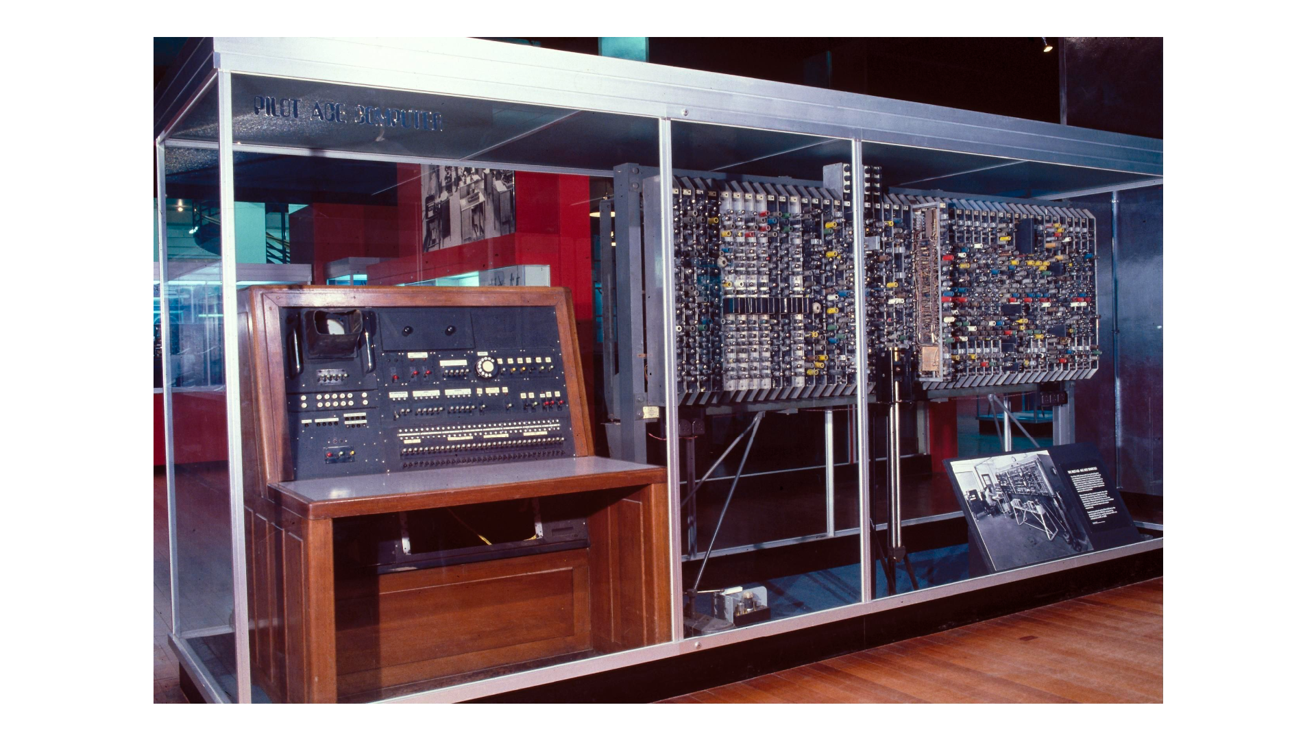
The Pilot ACE was a cut-down version of Turing’s full ACE design and originally intended to be a prototype, but it was quickly realised that this was a practical useable machine. It was subsequently upgraded and went into operation service for a few years until it was eventually shut down in May 1955 and given to the Science Museum in London, where it remains today.

The machine used around 800 valves (vacuum tubes) and it’s memory consisted of mercury delay lines which could store 128 words of 32 bits each originally, but this was later expanded in size. It ran at a clock rate of 1 megahertz, astonishingly fast for one of the earliest computers!

If you are used to programming a computer (probably since the 1960s), you’re probably used to being able to access RAM (random access memory) without having to know how long it would take to get a particular piece of data or your next program line out. It doesn’t make any difference if you’re asking for the first bit of data, the last or something in between. Not so for the Pilot ACE, the delay lines are sequential access memory, you need to wait an amount of time until the data you need is ready to be output from the delay line. This makes both the hardware design and how you write software quite different to how you might expect.

Mercury Delay Lines

The memory of the Pilot ACE used mercury delay lines. This type of delay line is basically a long tube, filled with mercury with a piezoelectric quartz crystal at one end and a receiver at the other. A bit to be stored was entered via the crystal as an acoustic pulse which travelled along the tube (1450 m/s in mercury) and was received at the other end after a small delay. When a pulse was received, this was amplified and then retransmitted at the start of the tube again meaning the data is stored indefinitely if you continue to retransmit the data.

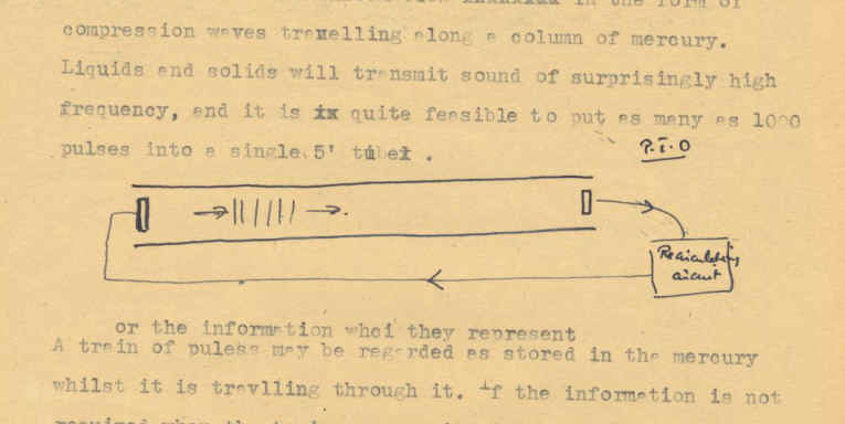
Given a precisely sized tube, it was then possible to store multiple bits of data within a tube with each being received one after the other at the far end after a delay and then retransmitted in the same order. The Pilot Ace’s word length was 32 bits so 32 pulses of audio, spaced at 1 microsecond apart, could be travelling along a single delay line at any time. To read the required word, you needed to wait up to 31μs for the first bit of data to be emerging from the tube. A longer delay line which could store 1024 bits of data (32 x 32 bits with a full cycle time of 1024μs) was also created with a correspondingly longer period to wait for the specific word of data to arrive at the output as well as a double size (64 bit) tube. On the Pilot ACE, a single 32μs timescale was called a minor cycle (mc) while the longer 1024μs of the long tubes was known as a major cycle (Mc).

History

The Pilot ACE was first run in 1950 and ended it's life in 1956, but during it's work at NPL, it went through several changes, especially with the console.

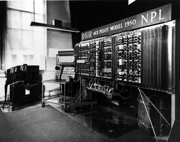
Pilot ACE - 1950

The initial Pilot ACE from 1950 is shown here, you can see that some of the computer is not yet completed. The console to control the computer is to the left on a trolley. It includes the basic Input / Output bulbs and switches at the top and the oscilloscope display below that to the left and the main console to the right. At this time, both separate units. The Hollerith comparitor allowing reading and punching of cards is the device in the far left of the photo.

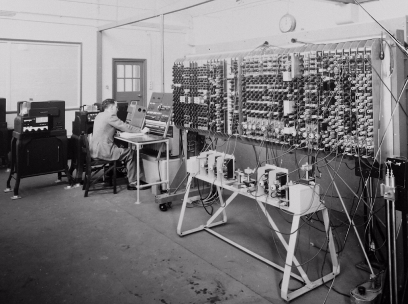
Pilot ACE - 1952

By 1952, the computer has got the majority of it's valves fitted and the beginnings of the console as we see it today at the Science Museum in London are seen. The short and double delay lines can be seen on the stand below the main computer as well as one of the long delay lines just visible on the floor at the far right of the photo. The scope output is still on a square unit to the left of the main console where the user is sitting.

Some more fantastic images of this period can be seen here Daily Mirror feature on the Team at the National Physical Laboratory.

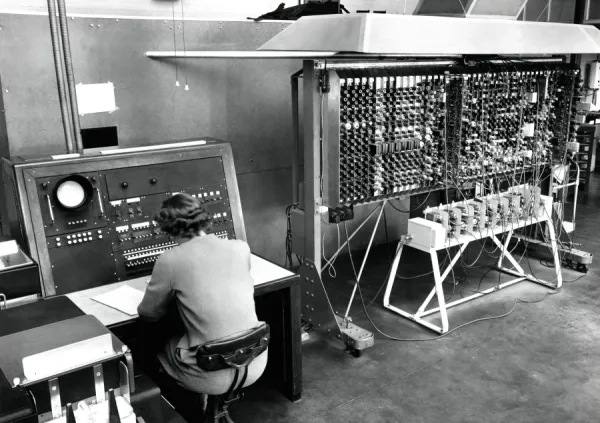
By late 1952-1953, the console has been completed with the new in-built oscilloscope and keys shown here. The options below the numeric keys though is still blank as this is the rotating drum memory setting which has yet to be built.

Pilot ACE - 1954

In 1954, the Pilot ACE received a drum memory with an additional 4096 words.

Pilot ACE - 1955

The Pilot ACE was so successful, that a commercial version, the DEUCE was constructed and sold by the English Electric Company selling a total of 33 units. The Pilot ACE was decommissioned in 1955 and given to the Science Museum where it can still be seen today.

System Design

If you have ever programmed assembler or machine code from nearly any modern computer since the 1960s, you’re probably used to a command structure in the format Function then Address, eg LDA 99, STA 100 or ADD 50, but the Pilot ACE is very much the exception to this and has a very different style of command structure.

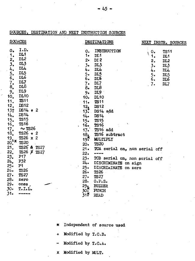
The standard command always has a source and a destination with each command doing a transfer from one to the other plus the time to wait until starting the transfer, the time to wait after the command and where to collect the next instruction. You can see a list of these sources and destinations here as found on “The Logical Design of the Pilot Model ACE, by J.H. Wilkinson” written in 1951.

The idea of this command structure is to minimise the time spent waiting for the next instruction or piece of data to emerge from the delay lines. Other computers of the time (EDSAC or EDVAC for example) just waited for the next instruction to emerge from a delay line meaning that a lot of time was spend with the computer doing nothing but waiting for data. Not so with the Pilot ACE, but this also added a huge amount of complexity to the programming stage!

The main stores consisted of ten long delay lines (DL1 – DL10) which, as stated above, held 32 words each of 32 bits which cycled at 1024μs (or 32mc). There were also six “temporary stores” (TS11, TS15, TS16, TS20, TS26 and TS27) which each held a single 32-bit word and two “double stores” (DS12 and DS14) which held two 32-bit words.

To transfer a word from TS11 to TS15 for example you would just specify the command with source 11 to destination 15. You could also do this in reverse by asking to transfer from 15 - 11.

If you wanted to copy all 32 of the words on the long delay line 1 onto delay line 4, you could just set a command to do DL1 – DL4 and repeat this for 32mc in a single command. This obviously only works if you want to transfer to another delay line into the same mc as the original. It gets a little more complex if you need to transfer just a single word of DL1 to a different delay line but want to store it in a different mc. To do this, you would use one of the temporary stores. First, we run a transfer from DL1₅-TS11 (the fifth word on delay line 1 so we start at 5 mc for 1 mc), then wait until we are at the mc required to store into the new delay line and do a transfer back, eg TS11-DL4₁₁.

As well as the delay line sources and destinations, there are also several “functional” sources that perform some logical and arithmetic functions. For example, TS16 has an adder-subtractor assigned to it, writing to destination 16 would just simply overwrite the value in TS16, but sending a source to 17 would add that source to the value in TS16. Likewise, sending to destination 18 would subtract that value.

The benefit of this format can be seen when we recall that each command contains the timing information so we can ask the computer to run the same command multiple times in one single command. We might want to add the number in TS15 to TS16 twelve times in a row. To do this on a more standard programming language, we’d probably need a loop to do this.

Example of adding a number 12 times with modern coding standards

1 COUNTER = 12
2 add TS15
3 decrement COUNTER
4 IF COUNTER > 0 JUMP 2
5 store TS16

On another delay line computer, each of these commands would be read from memory before being run with each pausing and waiting for the right time for the next command to emerge.

On Pilot ACE though, this command can be run in one single line which means only one single load from memory, and it will then run in the next 12 mc with no waiting at all. This could make a substantial speed difference when running commands based on a sequential program.

The same example on Pilot ACE

mc0 15-17 (12mc)

Optimal coding gave the Pilot ACE quite a speed advantage over the other machines of the time (at least when running the software). This is a comparative performance table from M.Campbell-Kelly's document giving benchmark times in ms to complete both a test benchmark program and general floating point operations. This shows that Pilot ACE was very fast for its time, but I suspect, due to the added complexity of Optimal Coding, while the actual runtime was much shorter, if you take into account the time to program and debug each system, there would be a different overall comparison.

Instruction Format

As mentioned above, the full instruction format, as well as the source and destination, included several other items including where to get the next instruction as well as timing information. Instead of placing instructions sequentially in consecutive storage locations, each instruction was placed in the store so that the next one would emerge from a delay line at precisely the moment that the last one was completed. In theory, this method could eliminate all the waiting time associated with collecting instructions and this technique was known as “optimum coding”. This method was very much functionality over usability though as it very much increases the complexity of the programming and debugging but very much increased the speed when running the program.

Each instruction took 2mc to begin with the instruction being placed into the TS COUNT delay line (the instruction store) then at 1mc after that, the source output would be opened to the highway followed by the destination input at 2mc.

Each complex instruction was fitted into a 32-bit word as follows:

N = Next instruction source; This was the DL to get the next instruction from eg 1 would get the next instruction from DL1. The timing for which instruction to get was based on the timing number T.
S = Source; This is the source delay line to open to transfer from given as a 5-bit number (0-31)
D = Destination; This is the destination for the transfer
s = Serial digit; If the serial digit was a 1, then the transfer would only ever run for a single minor cycle irrespective of the wait and timing fields. If 0, then the command would run repeatedly until the timing command end.
W = Wait number; The number of minor cycles to wait until beginning the transfer.
T = Timing number; The number of minor cycles to terminate the transfer.
X = go digit; If the go digit was a 1, then the instruction executed automatically, but if a 0, then the instruction would wait until a “one-shot” had been given, either by a manual switch on the console or by an instruction from the input/output devices.

The Wait and Timing options need a little further explanation! Each instruction took 2 mc to load and be ready to run, so both the Wait and Timing values are relative to the current mc of the instruction + 2. If, as in the example, the command being loaded is in 16mc which we’ll call m, then it will be ready in m+2 which is 18mc. Next, it will wait for 2mc as per the W digit (m + W + 2) before opening the destination gate and the transfer will begin.

This will then continue to run (as the serial bit is 0) for 5mc (T – W + 1) until it gets to the time of the Timing number (m + T + 2), the end time being irrespective of the value of W.

The next instruction, therefore, will be collected from the instruction source N at this time (m + T + 2) which in our example will be from 4₂₄.